Statistical distributions — numbers shaped like real life

A plain <gen type="number" value="150..200"/> draws uniformly — 150 is exactly as likely as 175 or 199. Real data almost never looks like that. People's heights cluster around an average, salaries are skewed (lots of middling ones, a few enormous), and wealth has a long, heavy tail. To generate believable numbers, add a distribution attribute to the number generator.

How to switch it on

There's no new tag — distribution is an attribute on the familiar <gen type="number">:

<gen type="number" distribution="normal" mean="170" sd="10"/>

The moment distribution="..." is present, the generator flips from range mode to distribution mode. Leave it off and the generator behaves exactly as before.

Here are four columns, each drawn from a different distribution (seed demo, 8 rows):

<env count="8" seed="demo">
  <sequence name="Height"> <gen type="number" distribution="normal"      mean="170" sd="10"/></sequence>
  <sequence name="Salary"> <gen type="number" distribution="lognormal"   meanlog="10.8" sdlog="0.5"/></sequence>
  <sequence name="Pause">  <gen type="number" distribution="exponential" rate="0.5" decimals="1"/></sequence>
  <sequence name="Balance"><gen type="number" distribution="pareto"      alpha="1.5" xmin="1000"/></sequence>
</env>

./run life.tdc (8 rows)

156 cm | $29884  | 0.4 s | $1329
175 cm | $75675  | 0.0 s | $2337
179 cm | $35084  | 1.1 s | $3587
160 cm | $74516  | 3.2 s | $3130
178 cm | $65256  | 1.1 s | $3285
170 cm | $39817  | 0.4 s | $1664
159 cm | $107734 | 1.9 s | $8781
182 cm | $65121  | 1.4 s | $2924

Heights stay near 170, salaries skew to the right, pauses are almost always short, and the balance never drops below 1000 but occasionally spikes.

Example outputs are illustrative

The histograms and values below are what a typical run produces. Exact draws can differ by core version, but the shape each distribution guarantees is what stays fixed. Distributions are deterministic — same seed, same numbers.

Uniform vs. "like real life" — visible on a histogram

The problem. Staring at a column of numbers won't tell you whether they're flat or bunched up. Draw the shape instead: generate 300 "heights" two ways and sort them into bins. Each histogram row is a range; the # bars show how many values landed in it (the n / min / max footer gives the totals and the edges).

A plain range — value="150..200". The numbers spread evenly across the whole range: a height of 150 is as common as 175 or 199. That's not how people are built:

<gen type="number" value="150..200"/>

./run uniform.tdc (300 rows)

150 | ############################# 27
154 | ####################### 21
158 | ############################### 29
163 | ######################## 22
167 | ##################### 19
171 | ######################## 22
175 | ################### 18
179 | ################################## 31
183 | ############################# 27
188 | ##################################### 34
192 | ############## 13
196 | ######################################## 37
n=300  min=150  max=200

The same range, but distribution="normal" (center 175, spread 8). A bell appears: most heights sit near the center and thin out toward the edges — just like real people:

<gen type="number" distribution="normal" mean="175" sd="8"/>

./run normal.tdc (300 rows)

157 | ### 5
161 | ############# 19
165 | ###################### 33
169 | ####################################### 57
172 | ######################################## 59
176 | ########################## 39
180 | ################################## 50
184 | ################# 25
188 | #### 6
192 | ## 3
195 | ## 3
199 | # 1
n=300  min=157  max=203

The same 150–200 range, generated 20,000 times each way and counted.

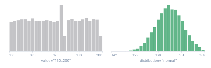
• a plain range: every height about as likely as any other
• the same range with a normal distribution: a hill around the center

The span of values is nearly the same (~150–200), but the shape is completely different: the uniform bars are all roughly the same height, while the normal ones form a hill peaking near 175 with rare edges. That's the whole point — moving from "uniform (unrealistic)" to "like real life."

All nine shapes, each generated with the attributes printed underneath. The horizontal axis stops at the 99th percentile — a long tail would otherwise squash every visible value into the first bar:

Nine runs of 8000 values each, counted. This is what the names actually look like.

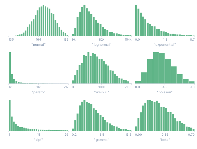
• 20,000 generated values, counted into buckets

normal — the bell curve

What it is. Values cluster around a center and get rarer the farther out you go, symmetrically on both sides. The classic bell-shaped curve.

Where it shows up. Height, weight, temperature, exam scores, measurement error — anything that wobbles around a typical value.

Parameters. mean — the center (average). sd — the spread (standard deviation: how widely values fan out from the center). Rule of thumb: about two-thirds of values fall within mean ± sd.

<gen type="number" distribution="normal" mean="170" sd="10"/>

./run normal.tdc (300 rows)

147 | #### 6
153 | ################# 28
159 | ################################## 55
164 | ######################################## 65
170 | ################################### 57
176 | #################################### 59
182 | ############# 21
188 | ### 5
193 | ## 3
199 | # 1
n=300  min=147  max=205

→ heights in centimeters: most between 160 and 180, rarely 150 or 190. A symmetric bell peaking near 170.

When to use it. A column like "height", "weight", or "temperature" — any quantity with a typical value and a symmetric spread around it.

lognormal — skewed to the right

What it is. Like normal, but tilted to the right: lots of small values and a long tail of large ones. Never negative.

Where it shows up. Salaries, prices, city sizes, session lengths — anywhere there's "a lot of ordinary, a little enormous."

Parameters. meanlog and sdlog are the center and spread of the logarithm of the value (that's how statisticians define this distribution). In practice: a larger meanlog makes the typical value bigger; a larger sdlog makes the rich tail longer. A useful anchor: the typical value is roughly e^meanlog, so meanlog=10.8 puts it around 49,000.

<gen type="number" distribution="lognormal" meanlog="10.8" sdlog="0.5"/>

./run lognormal.tdc (300 rows)

 15633 | ######################################## 114
41886 | ####################################### 110
68140 | ################## 51
94393 | ###### 17
120646 | # 3
146900 | # 1
173153 | # 2
199406 | # 1
225659 |  0
251913 | # 1
n=300  min=15633  max=278166

→ salary: a crowd around 50,000, a few earning far more. The peak is on the left with a long tail stretching right (to ~278,000).

When to use it. "Salary", "price", "file size" — quantities that can't go negative and skew toward large values.

exponential — time between events

What it is. The gaps between random events: many short ones, the occasional long one. Always non-negative.

Where it shows up. Time between orders, between clicks, between server failures, between calls to a call center.

Parameters. rate (the Greek λ) — how many events happen on average per unit of time. The mean wait is 1 / rate. With rate=0.5, events arrive roughly once every 2 units, so a typical pause is around 2.

<gen type="number" distribution="exponential" rate="0.5"/>

./run exponential.tdc (300 rows)

 0 | ############################ 70
1 | ######################################## 98
2 | ################### 47
3 | ################ 38
4 | ####### 17
5 | ####### 18
6 | # 3
7 | # 3
8 | # 2
9 | # 1
10 | # 2
12 | # 1
n=300  min=0  max=12

→ "seconds to the next event": usually a little, sometimes a lot. The tallest bar is at the low end and it falls off from there — short gaps are the most common.

When to use it. Any "how long until…" / "interval between…" column.

pareto — the 80/20 rule, long tail

What it is. Extreme skew: nearly every value is small, but the rare ones are huge. This is the "20% of causes produce 80% of effects" principle.

Where it shows up. Wealth (a few people own almost everything), video views, file sizes, city populations, follower counts.

Parameters. xmin — the smallest possible value (nothing falls below it). alpha — the tail thickness: the smaller alpha is, the fatter the tail (more rare giants). Around alpha 1–2 the tail is very pronounced.

<gen type="number" distribution="pareto" alpha="1.5" xmin="1000"/>

./run pareto.tdc (300 rows)

 1002 | ######################################## 259
4234 | #### 23
7466 | # 8
10698 | # 5
13930 | # 1
17162 |  0
20393 | # 1
23625 | # 2
26857 |  0
30089 | # 1
n=300  min=1002  max=33321

→ "account balance": everyone has at least 1000, but a handful have many times more. Almost all of it (259 of 300) sits in the first bin, while rare giants stretch out to ~33,000 — the classic long tail.

When to use it. Quantities where a few instances dominate the rest: money, popularity, sizes.

weibull — time to failure, reliability

What it is. A flexible "time to an event" distribution: unlike exponential (where risk is constant), here risk can rise or fall over time. One parameter sets the shape.

Where it shows up. How long a part lasts before it breaks, time to equipment failure, wind speeds, particle sizes.

Parameters. shape: shape < 1 is "infant mortality" (fails early or lasts a long time); shape = 1 behaves like exponential (constant risk); shape > 1 is wear-out (the longer it runs, the likelier it fails). scale — the characteristic time scale (roughly the typical time to failure).

<gen type="number" distribution="weibull" shape="1.5" scale="1000"/>

./run weibull.tdc (300 rows)

  30 | ########################## 57
358 | ######################################## 88
687 | ##################### 47
1015 | ######################## 52
1343 | ########## 21
1672 | ########## 23
2000 | ### 6
2328 | # 2
2656 | # 3
2985 | # 1
n=300  min=30  max=3313

→ "hours to failure": usually hundreds to thousands, with wear-out. At shape=1.5 the peak isn't pinned at zero (as it is for exponential) — it's shifted right: risk climbs first, then the tail falls off.

When to use it. Any "time in service until failure" / "time to an event" where risk isn't constant over time.

poisson — event counts

What it is. How many random events happened in an interval. A whole number. Values cluster around the average, but these are counts (0, 1, 2, 3…), not a continuous quantity.

Where it shows up. Calls to a call center per hour, defects per batch, emails per day, goals per match, visitors per minute.

Parameters. lambda — the average number of events per interval. With lambda=4 you usually get 2–6 events, occasionally 0 or 8+.

<gen type="number" distribution="poisson" lambda="4"/>

./run poisson.tdc (300 rows)

 0 | #### 5
1 | ############ 17
2 | #################################### 50
3 | ####################################### 53
4 | ##################################### 51
5 | ######################################## 55
6 | #################### 28
7 | ############### 21
8 | ########## 14
9 | ### 4
10 | # 2
n=300  min=0  max=10

→ "calls per hour": 3, 0, 7, 5, 3… These are counts (integers), peaking at the average lambda=4, spreading out both ways but never below 0.

Limitation. lambda is capped at 700. For very large averages, use normal with mean=lambda and sd ≈ the square root of lambda — the standard approximation.

When to use it. Any "how many times did it happen in a period" column.

zipf — ranked data, "stars and a long tail"

What it is. A few "stars" (rank 1, 2, 3…) appear very often, while a huge tail of rare ones almost never does. It returns a rank number (1, 2, … n).

Where it shows up. Word frequency in a language, website popularity, cities by population, follower counts, product sales.

Parameters. n — how many ranks there are (say 100 products). s — the "steepness": a larger s skews harder toward the first ranks. At s≈1 this is the classic Zipf's law.

<gen type="number" distribution="zipf" n="100" s="1.1"/>

./run zipf.tdc (300 rows)

 1 | ######################################## 174
11 | ########## 42
20 | ###### 27
30 | ### 12
39 | # 4
49 | ### 11
59 | ## 7
68 | ## 8
78 | ## 9
87 | # 6
n=300  min=1  max=97

→ "product rank": #1–#5 most often, #58 or #37 rarely. The first ranks take almost everything (174 of 300 are ranks 1–10); the other 90 positions are a rare long tail.

When to use it. When you need to model "the top dominates" — a pick from a numbered list where the first few positions account for nearly everything.

gamma — total waiting time

What it is. A generalization of exponential: if exponential is the time until one event, gamma is the total time until several. Always non-negative, skewed to the right.

Where it shows up. Time to accumulate N events, insurance payouts, rainfall totals, queue sizes, service response times (a sum of stages).

Parameters. shape (k) — "how many stages/events are summed" (a larger shape makes the peak more symmetric and pushes it right). scale (θ) — the scale. The mean is roughly shape · scale.

<gen type="number" distribution="gamma" shape="2" scale="1000"/>

./run gamma.tdc (300 rows)

  71 | ############################ 53
803 | ######################################## 77
1534 | ############################# 56
2266 | ############################# 55
2997 | ######### 18
3729 | ######### 17
4460 | ###### 11
5192 | #### 8
5923 | # 2
6655 | ## 3
n=300  min=71  max=7386

→ "milliseconds of waiting": usually around 2000 (2·1000), with a tail. Unlike exponential, the peak isn't pinned to zero — it's shifted right, because it's the sum of two stages.

When to use it. Total times or volumes that are the sum of several random contributions.

beta — fractions and probabilities (a number from 0 to 1)

What it is. The only distribution here whose values are always between 0 and 1. Two parameters set the shape (where the peak sits, how symmetric it is).

Where it shows up. Fractions, percentages, probabilities, conversion rates, 0–1 ratings, defect rates.

Parameters. alpha and beta pull mass toward 1 and toward 0 respectively. alpha = beta is symmetric around 0.5; alpha < beta skews toward zero (like a low conversion rate); alpha > beta skews toward one. The mean is roughly alpha / (alpha + beta).

<gen type="number" distribution="beta" alpha="2" beta="8" decimals="3"/>

Because the values all sit between 0 and 1, the bin labels on the left round to 0 — check the min/max footer for the real span (0.008..0.583):

./run beta.tdc (300 rows)

0 | ######################## 35
0 | ######################################## 59
0 | ################################# 49
0 | ############################### 46
0 | ################################# 48
0 | ############## 21
0 | ############ 18
0 | ######### 14
0 | #### 6
1 | ### 4
n=300  min=0.008  max=0.583

→ "conversion rate": usually 0.05–0.4 (mean ≈ 0.2). Everything is clamped to 0..1, the peak is near 0.2, and almost nothing reaches 1. Because the values are fractional, set decimals — otherwise they round to 0 or 1.

When to use it. Any fraction in the 0..1 range: a probability, a percentage, a conversion rate, a rating.

Controlling the output: decimals, min, max

decimals — digits after the decimal point

The default is 0 — the value rounds to a whole number (a height of "170", not "170.4213"). Ask for fractions explicitly:

<gen type="number" distribution="exponential" rate="1" decimals="3"/>   <!-- e.g. 0.693 -->

This matters most for beta (whose values live in 0..1) and for any time or ratio where whole-number rounding would flatten the detail.

min / max — clipping to bounds

Distributions occasionally emit extreme values (a normal with a small mean can go negative). min / max keep the value inside bounds: anything below min is pinned to min, anything above max is pinned to max.

<gen type="number" distribution="normal" mean="30" sd="20" min="0"/>   <!-- age is never negative -->

You can see it on the histogram. Without min, a normal with mean=30 sd=20 dips into negative territory (min=-16):

./run age-raw.tdc (300 rows)

-16 | ### 6
-4 | ############### 27
7 | ############################## 52
19 | ################################## 60
30 | ######################################## 70
42 | ############################### 55
53 | ############ 21
65 | ## 4
76 | ## 4
88 | # 1
n=300  min=-16  max=99

With min="0", everything that was below zero is pinned to zero — the left edge is exactly 0, and the zero bin swells (it absorbs the former negatives):

./run age-clipped.tdc (300 rows)

 0 | ################################# 46
10 | ################################# 46
20 | ####################################### 53
30 | ######################################## 55
40 | ####################################### 54
50 | ####################### 31
59 | ###### 8
69 | ## 3
79 | ## 3
89 | # 1
n=300  min=0  max=99

Both attributes are optional. Without them you get the raw distribution. Use them when a column has a hard floor or ceiling — an age, a percentage capped at 100, a non-negative amount.

The same generator, unbounded and bounded. Values that fall outside are pinned to the nearest bound, so the edges gain a spike.

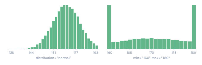
• left: no bounds; right: the same run bounded to 160 and 180

What you can't combine

distribution replaces the ordinary number mode, so you can't put it on the same generator as a range or percentages — TDC reports it plainly:

• value (a range), percent, length, include, and exclude are all incompatible with distribution — error TDC088:

./run bad.tdc

error[TDC088]: <gen type="number" distribution="..."> cannot be combined with "value"
note: A distribution replaces the range/percent. Remove "value", or drop "distribution" to use a range.

• An unknown distribution name, or a missing required parameter (e.g. normal without sd), is error TDC089 with a hint about what's needed:

./run bad.tdc

error[TDC089]: distribution "normal": "sd" is required and must be a number
note: Distributions: normal (mean, sd), lognormal (meanlog, sdlog), exponential (rate), pareto (alpha, xmin). Optional: decimals, min, max.

Determinism and scale

Like everything in TDC, distributions are deterministic: the same seed gives the same result. And they work at any volume — each row's value is computed from its row number, so memory doesn't grow with the number of rows (see Large outputs). A billion lognormal "salaries" is no problem.

All nine distributions are ready: normal, lognormal, exponential, pareto, weibull, poisson, zipf, gamma, and beta — exact, deterministic, and streamable at any scale.

See also

• Number — the range and digit-string modes this attribute replaces.
• Large outputs — why distributions stay cheap at a billion rows.
• Coherent data — keeping generated fields consistent within a row.